【机器学习】二维高斯函数的理解
看了好久,终于弄懂了二维高斯函数。谈谈我的简单理解。
高斯函数也就是正态分布的密度函数。一维高斯函数我们在概统中学习过,其方程为
或者写为
其中代表中心(均值),表示分布的幅度(标准差),表示高度。
若要使得对求积分的值为1,则
绘制图形的代码如下:
def gauss(mu, sigma, a):
    return a * np.exp(-(x - mu)**2 / (2 * sigma**2))

x = np.linspace(-4, 4, 100)
plt.figure(figsize=(4, 4))
plt.plot(x, gauss(0, 1, 1), 'black', linewidth=3)
plt.plot(x, gauss(2, 2, 0.5), 'gray', linewidth=3)

plt.ylim(-.5, 1.5)
plt.xlim(-4, 4)
plt.grid(True)
plt.show()
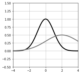
黑色线为, 灰色线为
到了二维,输入的就不只是了,而是
而高斯公式就变成了
对比一维
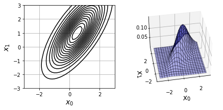
依然还是用三个变量用来控制二维高斯函数的形状:还是表示高度,表示均值向量(中心向量),表示函数分布的中心:
是协方差矩阵,是一个如下所示的矩阵:
中,和用来调整和方向分布的幅度(可以理解为两个一维分布中分别的)。$ \sigma _{01} 用于调整函数分布方向上的斜率,如果是正数,那么函数图形是右上左下方向↙️的椭圆;如果是负数,则是左上右下方向↘️的椭圆(x_0x_1$为纵轴的情况)。
简单起见,我们暂时设,然后计算。则可以发现,这个式子可以化成由和组成的二次型。
若要使得积分的值为1,则
其中
二维高斯函数的代码如下:
import numpy as np
import matplotlib.pyplot as plt
from mpl_toolkits.mplot3d import axes3d
%matplotlib inline

# 高斯函数 -----------------------------
def gauss(x, mu, sigma):
    N, D = x.shape
    c1 = 1 / (2 * np.pi)**(D / 2)
    c2 = 1 / (np.linalg.det(sigma)**(1 / 2))
    inv_sigma = np.linalg.inv(sigma)
    c3 = x - mu
    c4 = np.dot(c3, inv_sigma)
    c5 = np.zeros(N)
    for d in range(D):
        c5 = c5 + c4[:, d] * c3[:, d]
    p = c1 * c2 * np.exp(-c5 / 2)
    return p
绘图的代码如下所示:
X_range0=[-3, 3]
X_range1=[-3, 3]

# 显示等高线 --------------------------------
def show_contour_gauss(mu, sig):
    xn = 40  # 等高线的分辨率
    x0 = np.linspace(X_range0[0], X_range0[1], xn)
    x1 = np.linspace(X_range1[0], X_range1[1], xn)
    xx0, xx1 = np.meshgrid(x0, x1)
    x = np.c_[np.reshape(xx0, [xn * xn, 1]), np.reshape(xx1, [xn * xn, 1])]
    f = gauss(x, mu, sig)
    f = f.reshape(xn, xn)
    f = f.T
    cont = plt.contour(xx0, xx1, f, 15, colors='k')
    plt.grid(True)

# 三维图形 ----------------------------------
def show3d_gauss(ax, mu, sig):
    xn = 40  # 等高线的分辨率
    x0 = np.linspace(X_range0[0], X_range0[1], xn)
    x1 = np.linspace(X_range1[0], X_range1[1], xn)
    xx0, xx1 = np.meshgrid(x0, x1)
    x = np.c_[np.reshape(xx0, [xn * xn, 1]), np.reshape(xx1, [xn * xn, 1])]
    f = gauss(x, mu, sig)
    f = f.reshape(xn, xn)
    f = f.T
    ax.plot_surface(xx0, xx1, f,
                    rstride=2, cstride=2, alpha=0.3,
                    color='blue', edgecolor='black')

# 主处理 -----------------------------------
mu = np.array([1, 0.5])            # (A)
sigma = np.array([[2, 1], [1, 1]]) # (B)
Fig = plt.figure(1, figsize=(7, 3))
Fig.add_subplot(1, 2, 1)
show_contour_gauss(mu, sigma)
plt.xlim(X_range0)
plt.ylim(X_range1)
plt.xlabel('$x_0$', fontsize=14)
plt.ylabel('$x_1$', fontsize=14)
Ax = Fig.add_subplot(1, 2, 2, projection='3d')
show3d_gauss(Ax, mu, sigma)
Ax.set_zticks([0.05, 0.10])
Ax.set_xlabel('$x_0$', fontsize=14)
Ax.set_ylabel('$x_1$', fontsize=14)
Ax.view_init(40, -100)
plt.show()